HP 50g Calculator - The Basics of Plotting FunctionsPlotting on the HP 50gThe HP 50g calculator provides a host of plots to allow the user to visualize data or relationships between them. The white shifted-functions of the top row of keys on the HP 50g allow access to many of the input forms where plotting specifications may be entered. 2D/3D (PLOT SETUP) formThis example is performed in RPN mode. To set RPN mode:
The 2D/3D (PLOT SETUP) form is accessed by pressing left shift,
 , and simultaneously pressing and holding the
 (F4) key. When pressed, a form titled ‘PLOT SETUP’ is
displayed with a number of choices related to plotting as shown in
following figure.
(F4) key. When pressed, a form titled ‘PLOT SETUP’ is
displayed with a number of choices related to plotting as shown in
following figure.Figure 1: PLOT SETUP screen 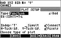
NOTE: To access the 'PLOT SETUP' form using an emulator, right-click left shift key, (
), followed by a left-click of
.The first option allows selecting the plot type
from a number of options. The selections for plot type are displayed by
pressing the
 menu key. The plot types include:
After pressing the
menu key, a choose box appears as shown below in Figure 2. Use the cursor keys to highlight the option and press
 . For this example, use the ‘Function’ option.
Figure 2: CHOOSE box 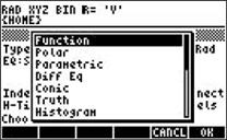
The ‘PLOT SETUP’ form also allows the user to
specify the equation being plotted. Place the cursor on the ‘EQ:’ field
using the cursor keys and press the
 menu label to invoke the EquationWriter used for constructing the equation to be plotted. See Figure 3.
Figure 3: EquationWriter 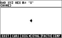
With the EquationWriter screen displayed, key in the desired equation using the keypad and the right-arrow cursor key (
 ) to move from one part of the equation to another. Press
 to input the equation.
For example, to enter y = x2-4, with ‘Function’ highlighted in the ‘PLOT SETUP’ screen, press:
This returns to the ‘PLOT SETUP’ screen with the equation in the 'EQ:' field. The form also allows to change the angle measure and the independent variable to be specified.
NOTE: The default is often 'X,' but for parametric plots, this will be changed to ‘t’.
For this example, be sure the independent variable (Indep:) is ‘X’. In addition, several check boxes indicate whether the plotted points should be automatically connected together by the calculator and the settings for the horizontal and vertical tick marks used for the graph. The form also allows for the plotting of more than one function at a time. For this example, leave all these settings in their defaults. The WIN formThe WIN form allows for the ‘PLOT WINDOW’ specifications to be entered and changed. The lower and upper horizontal and vertical values displayed on the graph can be changed. The lower and upper value for the independent variable can also be specified on this form. Use the arrow keys to move around the form. To open the WIN form, press
followed by the
 (F2) key.
Figure 4: PLOT WINDOW 
In the fields of the ‘PLOT WINDOW’ screen, enter the desired upper and lower values for the plot followed by
. For this example, set the x values from -3 to 3 (in the fields
'Indep Low:' and 'High:') and the y values -6 to 6 (in the fields
'H-View:' and 'V-View:'). With the ‘PLOT WINDOW’ displayed, and the cursor to the right of 'H-View:', press:
Figure 5: PLOT WINDOW with values entered 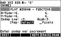
Once these parameters have been updated, press
 to discard the results of a previous plot, and
 to begin the plot. The plot should appear in the display as shown in the following figure. Note the new menu options.
Figure 6: PLOT 
What Can I Do with the Plot?
|


|
You are on HP Support Center for products such as printers, tablets, and desktops. |
|
|
For products such as servers, storage, and networking, go to HP Support Center - Hewlett Packard Enterprise . |